The calculation of the forced response of a DLIT system (see previous article) in response to u(k) input can be done by iteratively solving the difference equation of order n, or by resorting to the discrete convolution of the input with the impulse response of the system.
If the latter is not available, it can be derived by iteratively solving the difference equation with an input u(k)=δ(k) and null inputs and outputs for k<0.
In the case where the initial conditions are not null, it is possible to obtain y(k), given the sequence u(k) and the N values of the output prior to the instant k = 0, with a procedure very similar to that used for the solution of linear differential equations with constant coefficients for continuous systems over time.
Forced response and free-evolution of system
For the linearity of the system, you can consider the output y(k), for k≥0, as the sum of the forced response to the input signal starting from -M, and the free-evolution of the system, that is, u(k)=0 for every k and y(-1), y(-2), … y(-N) equal to the given initial values, namely:
![]()
The free evolution response ![]() can be calculated with:
can be calculated with:
![]()
This is called the associated homogeneous equation.
Characteristic equation
The general solution of the associated homogeneous equation is constructed from the roots of the characteristic equation:
![]()
If p is a simple root of the characteristic equation, it is easy to verify that the sequence ![]() satisfies the associated homogeneous equation.
satisfies the associated homogeneous equation.
Case of distinct roots
If C(λ)=0 has N distinct roots, the general solution of the homogeneous equation is given by the linear combination of linearly independent sequences ![]() , that is:
, that is:
![]()
The constants ![]() shall be calculated so that y(k) assumes the values given in k=-1….-N.
shall be calculated so that y(k) assumes the values given in k=-1….-N.
Case of root with multiplicity r and complex roots
In the case that the root p has multiplicity r, it contributes to the general solution ![]() with the linear combination of r linearly independent sequences:
with the linear combination of r linearly independent sequences:
![]() where j=0,1,2…r-1
where j=0,1,2…r-1
For r=3, we get the sequences ![]() ,
, ![]() ,
, ![]() .
.
In the case of simple but complex roots, they will be in complex conjugate pairs, since the coefficients of C(λ) are real, and in the same way the coefficients c must also be complex conjugates.
Solving difference equation: a basic example
![]()
It is a linear equation to the differences of order 1, in fact N = 1, M = 0.
The homogeneous equation results:
![]()
and the characteristic equation:
![]()
which has a single simple root a. The general solution then becomes:
![]()
If one wishes to evaluate the free evolution from the initial condition y(-1)=0.7, the coefficient c must be calculated so that:
![]()
which results:
![]()
We can also proceed through the calculation of the impulse response of the system. We can derive h(k) from the difference equation and it is:
![]()
where the factor ![]() is to make h(k) causal.
is to make h(k) causal.
The total response y(k), starting from a given value of y(-1) and with generic input u(k), is given by:
![]()
where the second term represents the forced response ![]() of the system.
of the system.
Consider now the latter with step input, i.e. ![]() :
:
![]()
When ![]() ,
, ![]() diverges, and when
diverges, and when ![]() it converges to the value
it converges to the value ![]() .
.
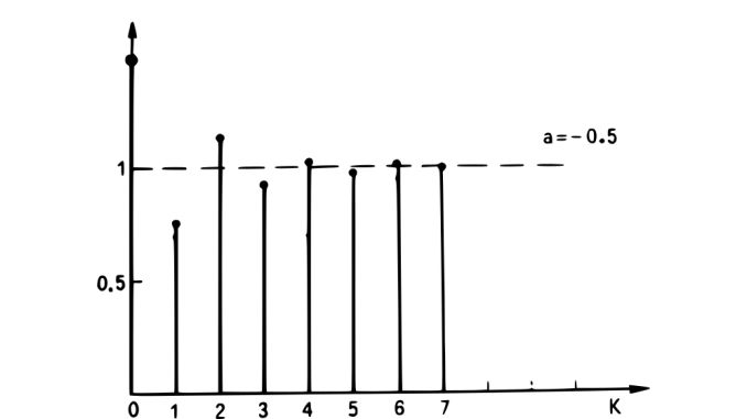
For ![]() the response is monotonous increasing, while for
the response is monotonous increasing, while for ![]() the response is oscillatory, as shown in the following figures in which (b=1-a) has been placed.
the response is oscillatory, as shown in the following figures in which (b=1-a) has been placed.
Solving difference equation: another example

Solution through impulse response
We determine the h(k) samples needed to calculate y(k) for k=0,1,2,3,4,5. That is, let’s determine the impulse response:
[1]To evaluate the samples h(k) we place in input a pulse: u(0)=δ(0)=1 and solve iteratively:

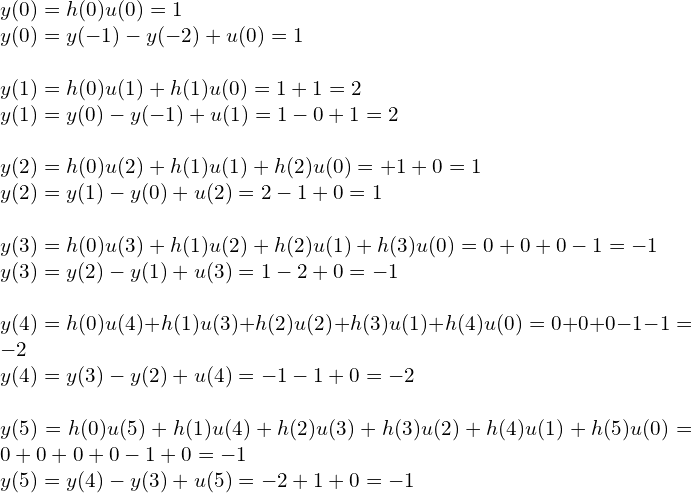
Iterative solution and comparison with the previous solution
Starting from:
![]()
we iteratively perform the calculation of the response and compare it with the previous solution, remembering [1].

As we can see, the results of the two methods coincide.


