This is the second part of a series of articles dedicated to digital filters. First part: Introduction to digital filters and comparison with analog filters.
The response over time to a constant input of an analog low-pass filter is typically the one shown in the figure:

As can be seen, it consists of an initial transient oscillatory type that dampens at full speed and is due to the action of the capacitor.
This transient, therefore, is a distinctive feature of the filter. Let’s see what happens when the delay due to the transient is comparable with the timing of variation of the input signal. Suppose you have a passive low-pass filter like:

in which we assume R=100 kΩ and C=10 nF; a time constant τ=10-3 s follows.
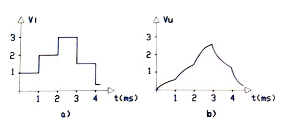
At the input of the filter we place a numerical signal, see figure 3a, with how much time T = 1 ms, or equal to the time constant of the filter. Assuming the capacitor is initially discharged, during the first period of the input it will begin to charge exponentially towards the voltage of 1 V. From the theory it is known that after a constant of time, that is, 1 ms, the capacitor will have reached 63% of the final value or 0.63 V.
After 1 ms, however, the input is brought to a value equal to 2 V: the capacitor then, which is charged at 0.63 V, will now charge towards a voltage equal to: (2 – 0.63)= 1.37 V. So after another millisecond the capacitor will be charged at a voltage equal to Vu = 0.63 (0.63×1.37) V = 1.49 V.
Iterating these calculations, we find that the output voltage of the filter follows the trend in figure 3-b. The effect of the filter is to smooth the edges of the input waveform: more precisely, the filter operates the moving average.

Moving average
Simply, the moving (weighted) mean of a series of discrete values can be expressed as:
![]()
where we assumed, for example, 3 values. The sum of the coefficients must be:
![]()
Mathematical model of an FIR digital filter
Generalizing what has been said above, the output of an FIR digital filter is obtained from the discrete convolution between the signal x(nT) and the distribution of the coefficients ai with how much time T = 1. We could demonstrate, in fact, that this discrete convolution is equivalent to a filtering operation in the time domain.
![]()
Expanding the equation to the previous finite differences, we can say that the output of an FIR filter of order N in the instant n, can be written as:
![]()
The output at a certain moment is therefore given by the linear combination of the input samples taken in a finite number of previous moments with certain coefficients, obtained by placing unit pulses in the input of the filter in the different instants. For this reason, this type of digital filter is called Finite Impulse Response (FIR).
Final comment
The behavior of a filter can be studied more comfortably in frequency by analyzing its transfer function. We will see it in the next part of this series of articles.


