
Digital control systems are now used predominantly, even where the processes to be controlled are analog.
The main reasons for this success stem from the inherent advantages of digital electronics: less circuit complexity, easier maintenance and the possibility of modifying the control logic without disrupting its structure. Not forgetting that digital signals ensure higher immunity to noise and low costs.
Consider, however, that some analog devices, such as transducers, actuators, and power amplifiers, cannot be replaced by similar digital components. This is therefore the need for a digital control system to involve the use of analog-to-digital converters – which convert analog signals into digital signals manipulated by control logic – and digital-to analog converters, which perform the reverse function, that is, convert digital control signals into analog signals that act on the process.
The functional aspect that characterizes digital controls compared to analog controls is the comparison node that, in the former, will be realized by a digital device that can vary from a simple comparator to a microprocessor board.
Microprocessor logics will naturally also find wide use in implementing the algorithms that define the regulator, from the simplest ON-OFF to the most complex obtained from the combination of proportional, derivative and integrative actions.
Figure 1 describes the general block scheme of a digital control applied to an analog process that uses an actuator and transducer. The signal emitted by the transducer is generally analog and is therefore continuous both in time and in amplitudes.
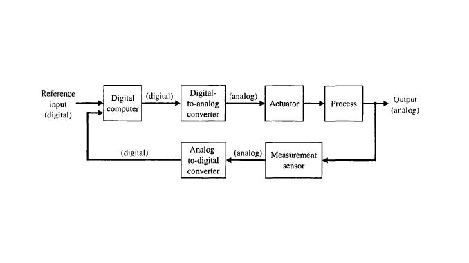
The microprocessor, however, is only able to operate at discrete time intervals, i.e. signal values are captured only at a few moments interspersed with each other by a fixed period T (sampling times). So if the signal is analog, it will have to be sampled in order to pick up its values only at certain moments that are equispatiated over time.
But sampling is not enough. In fact, to be managed by the microprocessor, they must also be discrete in amplitude: their values, that is, cannot assume the infinite possible values of an analog signal, but limit themselves to certain predetermined values within a certain range. The downstream sampling process, which “limits” the infinite continuous amplitude values to a finite and discrete subset, is called quantization.
In summary, quantization proceeds as follows:
- subdivision of the range of possible amplitude changes into subintervals;
- for each subinterval, a representative value is chosen, such as the average of the ends of the subinterval itself;
- replacement of the sampled amplitude value with the representative value of the sub-range to which it belongs.
For example, if the signal variation can fall in the range [-5,+5], subintervals could be: [-5,-4], [-4,-3], [-3,-2], [-2,-1], [-1,0], [0,+1], [+1,+2], [+2,+3], [+3,+4], [+4,+5].
Within these subintervals, representative values could be extreme averages, so: -4.5, -3.5, -2.5, -1.5, -0.5, +0.5, +1.5, +2.5, +3.5, +4.5.
Now, the values sampled at the various moments T, 2T, 3T etc. will be replaced with the representative values of the sample membership range. For example, if at instant T the sampled value is 2.8 V it would be replaced by quantization with a value of 2.5; the value 3.95 V replaced with 3.5; the value 4.6 V with 4.5, etc.
Quantization errors
It should be evident, at this point, that the quantization process involves an error, since the original “real” value is replaced by the quantized “approximated” value. You can immediately see that the maximum error will be equal to Q/2 where Q is the amplitude of the subinterval. In our example, where the subintervals had 1 V amplitude, the maximum quantization error will be 0.5 V.
It is already clear that it would be in our interest to build the smaller and smaller sub-intervals. In fact, if they had amplitude 0.1 V instead of 1 V, we would have reduced the maximum quantization error by 10 times: Q/2=0.05 V. However, we will see that this possibility has a limit that is dictated by another operation that must be carried out to make the signal manipulated by the microprocessor: Encoding. The latter must transform the chosen representative value (e.g. 3.5 V) into a binary number.
The set of the two quantization and coding operations is precisely that carried out by the analog-to-digital converters mentioned above. A more detailed block diagram of a digital control acting on three variables of an analog process is then that of Figure 2.

As shown in the figure, analog signals from transducers must pass through an conditioning circuit. The function of this circuit is to scale the signals of the transducers to the same amplitude range, for example [0, 10 V]. In this way they can be sent to the microprocessor one at a time on a single transmission line: this is the function of the analog multiplexer that follows the conditioning.
Proceeding along the transmission line, we find a low pass filter, a Sample and Hold circuit and finally the analog-to-digital converter (ADC).
The low pass filter has the function of limiting the influence of any high frequency disturbances on the signals.
The S/H circuit, Sample and Hold, operates as a kind of an analog memory: it keeps the value present at the ADC input constant for the duration of the conversion. The latter in fact takes a certain time (conversion time) and for it to succeed it has the need that the input value does not change before the conversion is finished.
Finally, the microprocessor, following a designed algorithm, processes the input signals and produces an output to intervene on the system to be controlled. Similar to the analog transmission line we have traveled, even at the output of the microprocessor you need a memory element that keeps the digital value that occurs at the input of the digital-analog converter (DAC) constant. This memory function is performed by a latch.
Proceeding in the diagram, the analog signal output from the DAC is sent to the power amplifier which, acting then on the actuator, allows the actuator to act on the controlled variable of the process, modifying it appropriately. Again, an S/H circuit is sometimes inserted in order to keep the input value of the power amplifier constant during its intervention on the actuator.
In a future article we will deal with control algorithms, seeing some examples in cases of PI and PID regulators.


